import torch
import torch.nn as nn
import torch.nn.functional as F
import torchvision
import torchvision.transforms as transforms
import numpy as np
from torch.utils.data import DataLoader, Dataset
import matplotlib.pyplot as plt
from PIL import Image
import random
from sklearn.decomposition import PCA
import os

# Set random seeds for reproducibility
torch.manual_seed(42)
np.random.seed(42)
random.seed(42)

# Check device
device = torch.device('cuda' if torch.cuda.is_available() else 'cpu')
print(f"Using device: {device}")

## SwAV Model Architecture

class SwAVModel(nn.Module):
    """
    SwAV model with ResNet-like backbone for CIFAR-10
    """
    def __init__(self, backbone_dim=512, num_prototypes=1000, projection_dim=128):
        super(SwAVModel, self).__init__()

        # CIFAR-10 optimized backbone
        self.backbone = nn.Sequential(
            # First conv block
            nn.Conv2d(3, 64, kernel_size=3, stride=1, padding=1),
            nn.BatchNorm2d(64),
            nn.ReLU(inplace=True),

            # Second conv block
            nn.Conv2d(64, 128, kernel_size=3, stride=2, padding=1),
            nn.BatchNorm2d(128),
            nn.ReLU(inplace=True),

            # Third conv block
            nn.Conv2d(128, 256, kernel_size=3, stride=2, padding=1),
            nn.BatchNorm2d(256),
            nn.ReLU(inplace=True),

            # Fourth conv block
            nn.Conv2d(256, 512, kernel_size=3, stride=2, padding=1),
            nn.BatchNorm2d(512),
            nn.ReLU(inplace=True),

            # Global average pooling
            nn.AdaptiveAvgPool2d((1, 1)),
            nn.Flatten()
        )

        # Projection head
        self.projection_head = nn.Sequential(
            nn.Linear(512, backbone_dim),
            nn.BatchNorm1d(backbone_dim),
            nn.ReLU(inplace=True),
            nn.Linear(backbone_dim, projection_dim)
        )

        # Prototypes (learnable cluster centers)
        self.prototypes = nn.Linear(projection_dim, num_prototypes, bias=False)

        # Initialize prototypes
        self.prototypes.weight.data.normal_(0, 0.01)
        self.prototypes.weight.data = F.normalize(self.prototypes.weight.data, dim=1)

    def forward(self, x):
        # Extract features
        features = self.backbone(x)

        # Project features
        z = self.projection_head(features)
        z = F.normalize(z, dim=1)

        # Compute prototype scores
        scores = self.prototypes(z)

        return z, scores

# Test model
model = SwAVModel()
print(f"Model parameters: {sum(p.numel() for p in model.parameters()):,}")

# Test forward pass
test_input = torch.randn(2, 3, 224, 224)
z, scores = model(test_input)
print(f"Feature shape: {z.shape}")
print(f"Scores shape: {scores.shape}")SwaV: Swapping Assignments between Views for Unsupervised Learning of Visual Features
self-supervised
contrastive-learning
vision
Exploring Swapping Assignments between Views for Unsupervised Learning of Visual Features
Introduction
SwAV (Swapping Assignments between Views) is a self-supervised learning method for visual representation learning introduced by Caron et al. in 2020.
Unlike contrastive methods that rely on negative sampling, SwAV adopts a clustering-based approach, encouraging consistency between cluster assignments from different augmentations of the same image.
Note
Read the original paper: Caron, Mathilde, et al.
Unsupervised Learning of Visual Features by Contrasting Cluster Assignments (SwaV) (2020)
arXiv:2006.09882
Key Concepts
1. Multi-Crop Strategy
SwAV introduces a multi-crop augmentation technique to expose the model to both global context and local details.
- Global crops: Two high-resolution crops of size 224×224
- Local crops: Several smaller crops, typically of size 96×96
This strategy increases data diversity without increasing batch size.
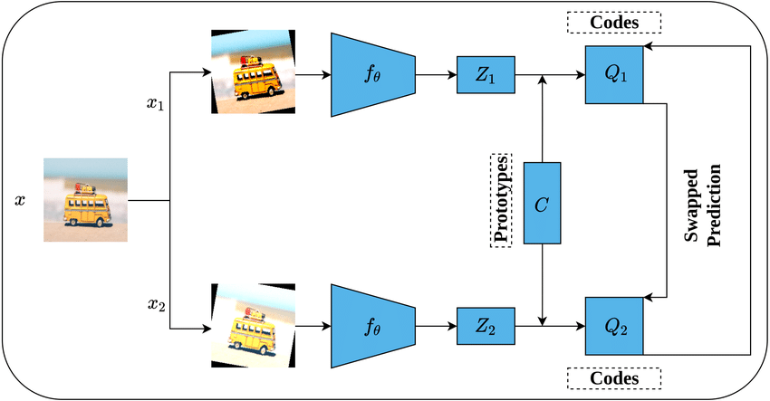
2. Clustering-Based Learning
Instead of comparing positive and negative pairs, SwAV:
- Maps input images to feature embeddings using a backbone network
- Assigns these embeddings to a set of learnable prototypes (i.e., cluster centers)
- Enforces consistency between the prototype assignments of different views (augmentations) of the same image
This avoids the need for explicit negative samples while encouraging invariant representations.
3. Sinkhorn-Knopp Algorithm
SwAV uses the Sinkhorn-Knopp algorithm to obtain balanced assignments to clusters.
This step solves an optimal transport problem, ensuring that each prototype receives approximately equal assignment probability, which helps prevent collapse (i.e., all embeddings mapping to the same cluster).
The algorithm normalizes the assignment matrix iteratively so that:
- Each row sums to 1 (each image maps to a probability distribution over prototypes)
- Each column sums to 1 (each prototype is used evenly across the batch)
This balanced soft-clustering technique is key to SwAV’s success without requiring contrastive loss.
Implementation
Sinkhorn-Knopp Algorithm
def sinkhorn_knopp(Q, num_iters=3, epsilon=0.05):
    """
    Sinkhorn-Knopp algorithm for optimal transport

    Args:
        Q: Matrix of prototype scores [batch_size, num_prototypes]
        num_iters: Number of iterations
        epsilon: Temperature parameter

    Returns:
        Normalized assignment matrix
    """
    Q = torch.exp(Q / epsilon)
    B, K = Q.shape

    # Make the matrix doubly stochastic
    for _ in range(num_iters):
        # Normalize rows (sum to 1 across prototypes)
        Q = Q / (Q.sum(dim=1, keepdim=True) + 1e-8)
        # Normalize columns (balanced assignments)
        Q = Q / (Q.sum(dim=0, keepdim=True) + 1e-8)
        # Rescale
        Q = Q * B

    return Q

# Test Sinkhorn-Knopp
test_scores = torch.randn(4, 10)
assignments = sinkhorn_knopp(test_scores)
print(f"Assignment matrix shape: {assignments.shape}")
print(f"Row sums: {assignments.sum(dim=1)}")
print(f"Column sums: {assignments.sum(dim=0)}")
SwAV Loss Function
class SwAVLoss(nn.Module):
    """
    SwAV loss function implementing the swapped prediction objective
    """
    def __init__(self, temperature=0.1, epsilon=0.05, sinkhorn_iterations=3):
        super(SwAVLoss, self).__init__()
        self.temperature = temperature
        self.epsilon = epsilon
        self.sinkhorn_iterations = sinkhorn_iterations

    def forward(self, z_list, scores_list):
        """
        Compute SwAV loss for multiple views

        Args:
            z_list: List of feature tensors from different views
            scores_list: List of prototype scores from different views
        """
        total_loss = 0
        num_views = len(z_list)

        for i in range(num_views):
            for j in range(num_views):
                if i != j:
                    # Get assignments from view i
                    with torch.no_grad():
                        q_i = sinkhorn_knopp(
                            scores_list[i],
                            self.sinkhorn_iterations,
                            self.epsilon
                        )

                    # Get predictions from view j
                    p_j = F.softmax(scores_list[j] / self.temperature, dim=1)

                    # Cross-entropy loss
                    loss = -torch.mean(torch.sum(q_i * torch.log(p_j + 1e-8), dim=1))
                    total_loss += loss

        return total_loss / (num_views * (num_views - 1))

# Test loss function
loss_fn = SwAVLoss()
test_z = [torch.randn(4, 128) for _ in range(4)]
test_scores = [torch.randn(4, 10) for _ in range(4)]
test_loss = loss_fn(test_z, test_scores)
print(f"Test loss: {test_loss.item():.4f}")
CIFAR-10 Multi-Crop Dataset
class CIFAR10MultiCrop(Dataset):
    """
    CIFAR-10 dataset with multi-crop augmentation for SwAV
    """
    def __init__(self, train=True, download=True,
                 global_crop_size=224, local_crop_size=96, num_local_crops=6):
        # Load CIFAR-10 dataset
        self.cifar10 = torchvision.datasets.CIFAR10(
            root='./data',
            train=train,
            download=download,
            transform=None
        )

        # Global crop transforms (high resolution)
        self.global_transform = transforms.Compose([
            transforms.RandomResizedCrop(global_crop_size, scale=(0.4, 1.0)),
            transforms.RandomHorizontalFlip(p=0.5),
            transforms.ColorJitter(brightness=0.4, contrast=0.4, saturation=0.4, hue=0.1),
            transforms.RandomGrayscale(p=0.2),
            transforms.ToTensor(),
            transforms.Normalize((0.4914, 0.4822, 0.4465), (0.2023, 0.1994, 0.2010))
        ])

        # Local crop transforms (lower resolution)
        self.local_transform = transforms.Compose([
            transforms.RandomResizedCrop(local_crop_size, scale=(0.05, 0.4)),
            transforms.RandomHorizontalFlip(p=0.5),
            transforms.ColorJitter(brightness=0.4, contrast=0.4, saturation=0.4, hue=0.1),
            transforms.RandomGrayscale(p=0.2),
            transforms.ToTensor(),
            transforms.Normalize((0.4914, 0.4822, 0.4465), (0.2023, 0.1994, 0.2010))
        ])

        self.num_local_crops = num_local_crops

    def __len__(self):
        return len(self.cifar10)

    def __getitem__(self, idx):
        image, _ = self.cifar10[idx]  # Ignore labels for self-supervised learning

        # Generate 2 global crops
        global_crops = [self.global_transform(image) for _ in range(2)]

        # Generate multiple local crops
        local_crops = [self.local_transform(image) for _ in range(self.num_local_crops)]

        return global_crops + local_crops

# Create dataset and dataloader
train_dataset = CIFAR10MultiCrop(train=True, download=True)
train_loader = DataLoader(train_dataset, batch_size=32, shuffle=True, num_workers=2)

print(f"Dataset size: {len(train_dataset)}")
print(f"Number of batches: {len(train_loader)}")

# Visualize some crops
sample_crops = train_dataset[0]
print(f"Number of crops per image: {len(sample_crops)}")
print(f"Global crop 1 shape: {sample_crops[0].shape}")
print(f"Local crop 1 shape: {sample_crops[2].shape}")
Visualization of Multi-Crop Strategy
def visualize_multicrop_sample():
    """Visualize the multi-crop strategy on a CIFAR-10 sample"""
    # Get original CIFAR-10 image
    cifar10_orig = torchvision.datasets.CIFAR10(root='./data', train=True, download=False)
    orig_image, label = cifar10_orig[100]

    # Get multi-crop version
    crops = train_dataset[100]

    # Plot
    fig, axes = plt.subplots(2, 5, figsize=(15, 6))

    # Original image
    axes[0, 0].imshow(orig_image)
    axes[0, 0].set_title('Original\nCIFAR-10')
    axes[0, 0].axis('off')

    # Global crops
    for i in range(2):
        crop = crops[i]
        # Denormalize for visualization
        crop = crop * torch.tensor([0.2023, 0.1994, 0.2010]).view(3, 1, 1)
        crop = crop + torch.tensor([0.4914, 0.4822, 0.4465]).view(3, 1, 1)
        crop = torch.clamp(crop, 0, 1)

        axes[0, i+1].imshow(crop.permute(1, 2, 0))
        axes[0, i+1].set_title(f'Global Crop {i+1}\n224×224')
        axes[0, i+1].axis('off')

    # Local crops (first 6)
    for i in range(6):
        crop = crops[i+2]
        # Denormalize for visualization
        crop = crop * torch.tensor([0.2023, 0.1994, 0.2010]).view(3, 1, 1)
        crop = crop + torch.tensor([0.4914, 0.4822, 0.4465]).view(3, 1, 1)
        crop = torch.clamp(crop, 0, 1)

        row = 0 if i < 3 else 1
        col = (i % 3) + 2
        if row == 1:
            col = (i % 3)

        axes[row, col].imshow(crop.permute(1, 2, 0))
        axes[row, col].set_title(f'Local Crop {i+1}\n96×96')
        axes[row, col].axis('off')

    # Hide unused subplots
    for i in range(3, 5):
        axes[1, i].axis('off')

    plt.tight_layout()
    plt.show()

visualize_multicrop_sample()
Training Function
def train_swav(model, train_loader, num_epochs=10, lr=0.001):
    """
    Train SwAV model on CIFAR-10
    """
    model.to(device)
    optimizer = torch.optim.Adam(model.parameters(), lr=lr, weight_decay=1e-4)
    scheduler = torch.optim.lr_scheduler.CosineAnnealingLR(optimizer, T_max=num_epochs)
    criterion = SwAVLoss()

    model.train()
    losses = []

    print(f"Training SwAV on CIFAR-10 for {num_epochs} epochs")
    print(f"Device: {device}")
    print("-" * 60)

    for epoch in range(num_epochs):
        epoch_loss = 0
        num_batches = 0

        for batch_idx, crops in enumerate(train_loader):
            try:
                # Move crops to device
                crops = [crop.to(device) for crop in crops]

                # Forward pass through all crops
                z_list = []
                scores_list = []

                for crop in crops:
                    z, scores = model(crop)
                    z_list.append(z)
                    scores_list.append(scores)

                # Compute SwAV loss
                loss = criterion(z_list, scores_list)

                # Backward pass
                optimizer.zero_grad()
                loss.backward()
                torch.nn.utils.clip_grad_norm_(model.parameters(), max_norm=1.0)
                optimizer.step()

                # Normalize prototypes
                with torch.no_grad():
                    model.prototypes.weight.data = F.normalize(
                        model.prototypes.weight.data, dim=1
                    )

                epoch_loss += loss.item()
                num_batches += 1

                if batch_idx % 50 == 0:
                    print(f'Epoch {epoch+1}/{num_epochs}, Batch {batch_idx}/{len(train_loader)}, Loss: {loss.item():.4f}')

            except Exception as e:
                print(f"Error in batch {batch_idx}: {e}")
                continue

        scheduler.step()

        if num_batches > 0:
            avg_loss = epoch_loss / num_batches
            losses.append(avg_loss)
            print(f'Epoch {epoch+1} Complete - Avg Loss: {avg_loss:.4f}, LR: {scheduler.get_last_lr()[0]:.6f}')

        print("-" * 60)

    return losses

# Initialize model and start training
model = SwAVModel(backbone_dim=512, num_prototypes=500, projection_dim=128)
print(f"Model parameters: {sum(p.numel() for p in model.parameters()):,}")

# Train the model
losses = train_swav(model, train_loader, num_epochs=5, lr=0.001)
Results Visualization
plt.figure(figsize=(12, 5))

plt.subplot(1, 2, 1)
plt.plot(losses, 'b-', linewidth=2, marker='o')
plt.title('SwAV Training Loss on CIFAR-10')
plt.xlabel('Epoch')
plt.ylabel('Loss')
plt.grid(True, alpha=0.3)

# Extract features for visualization
model.eval()
feature_extractor = nn.Sequential(model.backbone, model.projection_head)

# Simple dataset for feature extraction
simple_dataset = torchvision.datasets.CIFAR10(
    root='./data', train=False, download=True,
    transform=transforms.Compose([
        transforms.Resize(224),
        transforms.ToTensor(),
        transforms.Normalize((0.4914, 0.4822, 0.4465), (0.2023, 0.1994, 0.2010))
    ])
)

simple_loader = DataLoader(simple_dataset, batch_size=100, shuffle=False)

# Extract features
features = []
labels = []

with torch.no_grad():
    for batch_idx, (images, batch_labels) in enumerate(simple_loader):
        if batch_idx >= 10:  # Limit to first 1000 samples
            break
        images = images.to(device)
        batch_features = feature_extractor(images)
        features.append(batch_features.cpu())
        labels.append(batch_labels)

features = torch.cat(features, dim=0).numpy()
labels = torch.cat(labels, dim=0).numpy()

# PCA visualization
pca = PCA(n_components=2)
features_2d = pca.fit_transform(features)

plt.subplot(1, 2, 2)
classes = ['plane', 'car', 'bird', 'cat', 'deer', 'dog', 'frog', 'horse', 'ship', 'truck']
colors = plt.cm.tab10(np.linspace(0, 1, 10))

for i, class_name in enumerate(classes):
    mask = labels == i
    plt.scatter(features_2d[mask, 0], features_2d[mask, 1],
               c=[colors[i]], label=class_name, alpha=0.6, s=20)

plt.title('SwAV Features PCA Visualization')
plt.xlabel('Principal Component 1')
plt.ylabel('Principal Component 2')
plt.legend(bbox_to_anchor=(1.05, 1), loc='upper left')
plt.grid(True, alpha=0.3)

plt.tight_layout()
plt.show()

print(f"Feature extraction completed: {features.shape[0]} samples, {features.shape[1]} dimensions")
Feature Quality Analysis
# Analyze feature quality
plt.figure(figsize=(15, 5))

# Feature distribution
plt.subplot(1, 3, 1)
plt.hist(features.flatten(), bins=50, alpha=0.7, color='skyblue')
plt.title('Feature Value Distribution')
plt.xlabel('Feature Value')
plt.ylabel('Frequency')
plt.grid(True, alpha=0.3)

# Feature variance across dimensions
plt.subplot(1, 3, 2)
feature_var = np.var(features, axis=0)
plt.plot(feature_var, 'g-', linewidth=2)
plt.title('Feature Variance per Dimension')
plt.xlabel('Feature Dimension')
plt.ylabel('Variance')
plt.grid(True, alpha=0.3)

# Feature correlation matrix (subset)
plt.subplot(1, 3, 3)
correlation_matrix = np.corrcoef(features[:, :32].T)  # First 32 dimensions
plt.imshow(correlation_matrix, cmap='coolwarm', vmin=-1, vmax=1)
plt.title('Feature Correlation Matrix\n(First 32 dimensions)')
plt.colorbar()

plt.tight_layout()
plt.show()

# Print statistics
print(f"Feature Statistics:")
print(f"Mean: {features.mean():.4f}")
print(f"Std: {features.std():.4f}")
print(f"Min: {features.min():.4f}")
print(f"Max: {features.max():.4f}")
Key Advantages of SwAV
- No Negative Sampling: Unlike contrastive methods, SwAV doesn’t require negative pairs
- Scalability: Works well with large batch sizes and many prototypes
- Multi-scale Learning: Uses crops of different sizes for better representation learning
- Balanced Assignments: Sinkhorn-Knopp ensures balanced cluster assignments
Comparison with Other Methods
| Method | Approach | Key Innovation |
|---|---|---|
| SimCLR | Contrastive | Large batch sizes + strong augmentation |
| MoCo | Contrastive | Momentum encoder + queue |
| SwAV | Clustering | Prototype-based assignments + multi-crop |
| BYOL | Non-contrastive | Predictor network + stop gradient |
Practical Considerations
- Prototype Initialization: Prototypes should be normalized and well-initialized
- Sinkhorn Iterations: Usually 3 iterations are sufficient
- Temperature Scaling: Important for balancing assignments
- Multi-crop Ratios: Typically 2 global + 6 local crops
Future Directions
SwAV has inspired several important follow-up works in self-supervised learning:
SeLa: Integrates SwAV-style clustering with momentum encoder updates for improved stability.
DenseCL: Adapts SwAV principles for dense prediction tasks such as object detection and segmentation.
SwAV+: Enhances the original SwAV with stronger augmentations and improved architectural choices.
This implementation serves as a strong foundation for understanding and experimenting with SwAV.
For real-world or production-level applications, consider using the official implementation, which includes robust ResNet backbones, better training schedules, and optimized performance settings.