# Required imports
import torch
import torch.nn as nn
import torch.nn.functional as F
import torchvision
import torchvision.transforms as transforms
from torch.utils.data import DataLoader, Dataset
import numpy as np
import matplotlib.pyplot as plt
from PIL import Image
import random
import os

# Set random seeds for reproducibility
torch.manual_seed(42)
np.random.seed(42)
random.seed(42)

device = torch.device('cuda' if torch.cuda.is_available() else 'cpu')
print(f'Using device: {device}')SimCLR: Simple Contrastive Learning of Visual Representations
self-supervised
contrastive-learning
vision
An in-depth look at SimCLR, a self-supervised learning framework that leverages contrastive learning to learn visual representations without labeled data.
Introduction
SimCLR (Simple Contrastive Learning of Visual Representations) is a self-supervised learning framework for learning visual representations without labels. It was introduced by Chen et al. in 2020 and has become one of the most influential methods in contrastive learning.
Note
Read the original paper: Chen, Ting, et al.
A Simple Framework for Contrastive Learning of Visual Representations (2020)
arXiv:2002.05709
Key Concepts
- Contrastive Learning: Learn representations by contrasting positive and negative examples.
- Data Augmentation: Create positive pairs through augmentation of the same image.
- Projection Head: Use a non-linear projection head during training.
- Large Batch Sizes: Utilize large batch sizes for more negative examples.
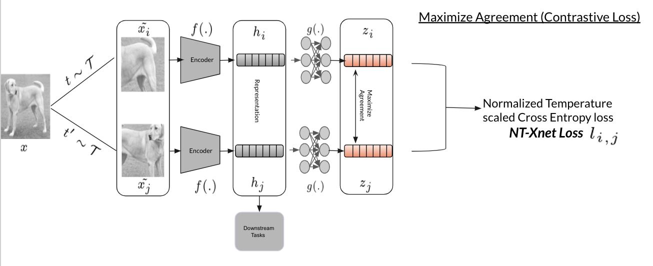
How SimCLR Works
- Take a batch of images.
- Apply two different augmentations to each image (creating positive pairs).
- Pass augmented images through an encoder (e.g., ResNet).
- Apply a projection head to get representations.
- Use contrastive loss (NT-Xent) to pull positive pairs together and push negative pairs apart.
Data Augmentation Pipeline
Data augmentation is crucial for SimCLR’s success. The framework uses a composition of augmentations to create positive pairs from the same image.
# Data Augmentation Pipeline
class SimCLRTransform:

    def __init__(self, image_size=224, s=1.0):
        self.image_size = image_size

        # Color distortion
        color_jitter = transforms.ColorJitter(
            brightness=0.8 * s,
            contrast=0.8 * s,
            saturation=0.8 * s,
            hue=0.2 * s
        )

        # SimCLR augmentation pipeline
        self.transform = transforms.Compose([
            transforms.RandomResizedCrop(image_size, scale=(0.08, 1.0)),
            transforms.RandomHorizontalFlip(p=0.5),
            transforms.RandomApply([color_jitter], p=0.8),
            transforms.RandomGrayscale(p=0.2),
            transforms.ToTensor(),
            transforms.Normalize(
                mean=[0.485, 0.456, 0.406],
                std=[0.229, 0.224, 0.225]
            )
        ])

    def __call__(self, x):
        # Return two augmented versions of the same image
        return self.transform(x), self.transform(x)

# Demonstration of augmentation
transform = SimCLRTransform()
print("SimCLR augmentation pipeline created")
SimCLR Model Architecture
The SimCLR model is built from two key components:
1. Encoder
- A deep convolutional neural network (CNN), such as ResNet, is used to extract feature representations from input images.
- The encoder learns to map images to a high-dimensional feature space that captures semantic content.
2. Projection Head
- A small multilayer perceptron (MLP) that takes the encoder’s output and projects it into a lower-dimensional space.
- This projection is where the contrastive loss is applied, encouraging similar images (positive pairs) to have similar representations and dissimilar images (negative pairs) to be far apart.
Key Points
- The projection head is used only during contrastive pre-training; for downstream tasks, only the encoder is retained.
- This separation improves the quality of learned representations and makes SimCLR simple yet powerful for self-supervised learning.
# SimCLR Model Architecture
class ProjectionHead(nn.Module):

    def __init__(self, input_dim=512, hidden_dim=512, output_dim=128):
        super().__init__()
        self.projection = nn.Sequential(
            nn.Linear(input_dim, hidden_dim),
            nn.ReLU(),
            nn.Linear(hidden_dim, output_dim)
        )

    def forward(self, x):
        return self.projection(x)

class SimCLR(nn.Module):
    """SimCLR model implementation"""

    def __init__(self, base_encoder='resnet18', projection_dim=128):
        super().__init__()

        # Base encoder
        if base_encoder == 'resnet18':
            self.encoder = torchvision.models.resnet18(weights=None)
            self.encoder.fc = nn.Identity()  # Remove classification head
            encoder_dim = 512
        elif base_encoder == 'resnet50':
            self.encoder = torchvision.models.resnet50(weights=None)
            self.encoder.fc = nn.Identity()
            encoder_dim = 2048
        else:
            raise ValueError(f"Unsupported encoder: {base_encoder}")

        # Projection head
        self.projection_head = ProjectionHead(
            input_dim=encoder_dim,
            output_dim=projection_dim
        )

    def forward(self, x):
        # Extract features
        features = self.encoder(x)
        # Project features
        projections = self.projection_head(features)
        return features, projections

# Create model
model = SimCLR(base_encoder='resnet18', projection_dim=128)
model = model.to(device)
print(f"SimCLR model created with {sum(p.numel() for p in model.parameters())} parameters")
NT-Xent Loss Function
The Normalized Temperature-scaled Cross-Entropy (NT-Xent) loss is the heart of SimCLR. It encourages similar representations for positive pairs while pushing apart negative pairs.
# NT-Xent Loss Function
class NTXentLoss(nn.Module):

    def __init__(self, temperature=0.07):
        super().__init__()
        self.temperature = temperature
        self.criterion = nn.CrossEntropyLoss(reduction='sum')
        self.similarity_f = nn.CosineSimilarity(dim=2)

    def mask_correlated_samples(self, batch_size):
        """Create mask to remove self-similarity and correlated samples"""
        N = 2 * batch_size
        mask = torch.ones((N, N), dtype=bool)
        mask = mask.fill_diagonal_(0)
        for i in range(batch_size):
            mask[i, batch_size + i] = 0
            mask[batch_size + i, i] = 0
        return mask

    def forward(self, z_i, z_j):
        """Calculate NT-Xent loss"""
        batch_size = z_i.shape[0]
        N = 2 * batch_size
        z = torch.cat((z_i, z_j), dim=0)
        sim = self.similarity_f(z.unsqueeze(1), z.unsqueeze(0)) / self.temperature
        sim_i_j = torch.diag(sim, batch_size)
        sim_j_i = torch.diag(sim, -batch_size)
        positive_samples = torch.cat((sim_i_j, sim_j_i), dim=0).reshape(N, 1)
        mask = self.mask_correlated_samples(batch_size)
        negative_samples = sim[mask].reshape(N, -1)
        labels = torch.zeros(N).to(positive_samples.device).long()
        logits = torch.cat((positive_samples, negative_samples), dim=1)
        loss = self.criterion(logits, labels)
        return loss / N

# Create loss function
criterion = NTXentLoss(temperature=0.07)
print("NT-Xent loss function created")
Custom Dataset for SimCLR
We’ll create a custom dataset class that applies SimCLR augmentations to create positive pairs.
# Custom Dataset for SimCLR
class SimCLRDataset(Dataset):
    """Dataset wrapper for SimCLR that returns augmented pairs"""

    def __init__(self, dataset, transform=None):
        self.dataset = dataset
        self.transform = transform

    def __len__(self):
        return len(self.dataset)

    def __getitem__(self, idx):
        image, _ = self.dataset[idx]
        # Note that labels are ignored for self supervised learning
        if self.transform:
            aug1, aug2 = self.transform(image)
            return aug1, aug2
        else:
            return image, image

# Load CIFAR-10 dataset (you can replace with your own dataset)
base_dataset = torchvision.datasets.CIFAR10(
    root='./data',
    train=True,
    download=True,
    transform=transforms.ToPILImage()
)

# Create SimCLR dataset
simclr_dataset = SimCLRDataset(base_dataset, transform=SimCLRTransform(image_size=32))
dataloader = DataLoader(simclr_dataset, batch_size=64, shuffle=True, num_workers=2)

print(f"Dataset created with {len(simclr_dataset)} samples")
print(f"Dataloader created with batch size {dataloader.batch_size}")
Training Loop
Now let’s implement the training loop for SimCLR. This demonstrates how the model learns representations through contrastive learning.
# Training Loop
def train_simclr(model, dataloader, criterion, optimizer, num_epochs=25):
    """Training loop for SimCLR"""
    model.train()
    losses = []
    for epoch in range(num_epochs):
        epoch_loss = 0.0
        num_batches = 0
        for batch_idx, (aug1, aug2) in enumerate(dataloader):
            aug1, aug2 = aug1.to(device), aug2.to(device)
            _, z1 = model(aug1)
            _, z2 = model(aug2)
            z1 = F.normalize(z1, dim=1)
            z2 = F.normalize(z2, dim=1)
            loss = criterion(z1, z2)
            optimizer.zero_grad()
            loss.backward()
            optimizer.step()
            epoch_loss += loss.item()
            num_batches += 1
            if batch_idx % 50 == 0:
                print(f'Epoch {epoch+1}/{num_epochs}, Batch {batch_idx}/{len(dataloader)}, Loss: {loss.item():.4f}')
        avg_loss = epoch_loss / num_batches
        losses.append(avg_loss)
        print(f'Epoch {epoch+1}/{num_epochs} completed. Average Loss: {avg_loss:.4f}')
    return losses

# Create optimizer
optimizer = torch.optim.Adam(model.parameters(), lr=3e-4, weight_decay=1e-6)

# Train the model
print("Starting SimCLR training")
losses = train_simclr(model, dataloader, criterion, optimizer, num_epochs=25)

# Plot training loss
plt.figure(figsize=(10, 6))
plt.plot(losses)
plt.title('SimCLR Training Loss')
plt.xlabel('Epoch')
plt.ylabel('Loss')
plt.grid(True)
plt.show()

print("Training completed")
Evaluation: Linear Probing
After pre-training with SimCLR, we typically evaluate the learned representations using linear probing—training a linear classifier on top of frozen features.
# Evaluation: Linear Probing
class LinearProbe(nn.Module):
    """Linear classifier for evaluation"""

    def __init__(self, feature_dim, num_classes):
        super().__init__()
        self.classifier = nn.Linear(feature_dim, num_classes)

    def forward(self, x):
        return self.classifier(x)

def evaluate_linear_probe(model, train_loader, test_loader, num_classes=10):
    """Evaluate learned representations using linear probing"""
    model.eval()
    train_features = []
    train_labels = []
    with torch.no_grad():
        for images, labels in train_loader:
            images = images.to(device)
            features, _ = model(images)
            train_features.append(features.cpu())
            train_labels.append(labels)
    train_features = torch.cat(train_features)
    train_labels = torch.cat(train_labels)
    linear_probe = LinearProbe(train_features.shape[1], num_classes).to(device)
    optimizer = torch.optim.Adam(linear_probe.parameters(), lr=1e-3)
    criterion = nn.CrossEntropyLoss()
    linear_probe.train()
    for epoch in range(10):
        indices = torch.randperm(len(train_features))
        for i in range(0, len(train_features), 256):
            batch_indices = indices[i:i+256]
            batch_features = train_features[batch_indices].to(device)
            batch_labels = train_labels[batch_indices].to(device)
            optimizer.zero_grad()
            outputs = linear_probe(batch_features)
            loss = criterion(outputs, batch_labels)
            loss.backward()
            optimizer.step()
    linear_probe.eval()
    correct = 0
    total = 0
    with torch.no_grad():
        for images, labels in test_loader:
            images = images.to(device)
            features, _ = model(images)
            outputs = linear_probe(features)
            _, predicted = torch.max(outputs.data, 1)
            total += labels.size(0)
            correct += (predicted.cpu() == labels).sum().item()
    accuracy = 100 * correct / total
    return accuracy

# Create evaluation datasets
eval_transform = transforms.Compose([
    transforms.Resize(32),
    transforms.ToTensor(),
    transforms.Normalize(mean=[0.485, 0.456, 0.406], std=[0.229, 0.224, 0.225])
])

train_eval_dataset = torchvision.datasets.CIFAR10(
    root='./data', train=True, download=False, transform=eval_transform
)
test_eval_dataset = torchvision.datasets.CIFAR10(
    root='./data', train=False, download=False, transform=eval_transform
)

train_eval_loader = DataLoader(train_eval_dataset, batch_size=256, shuffle=False)
test_eval_loader = DataLoader(test_eval_dataset, batch_size=256, shuffle=False)

# Evaluate
print("Evaluating learned representations")
accuracy = evaluate_linear_probe(model, train_eval_loader, test_eval_loader)
print(f"Linear probe accuracy: {accuracy:.2f}%")
Visualization: Feature Similarity
Let’s visualize how similar the learned features are for augmented versions of the same image.
# Visualization: Feature Similarity
def visualize_feature_similarity(model, dataset, num_samples=5):
    """Visualize similarity between features of augmented pairs"""
    model.eval()
    fig, axes = plt.subplots(num_samples, 3, figsize=(12, 4 * num_samples))
    if num_samples == 1:
        axes = axes.reshape(1, -1)
    with torch.no_grad():
        for i in range(num_samples):
            aug1, aug2 = dataset[i]
            aug1 = aug1.unsqueeze(0).to(device)
            aug2 = aug2.unsqueeze(0).to(device)
            _, z1 = model(aug1)
            _, z2 = model(aug2)
            z1 = F.normalize(z1, dim=1)
            z2 = F.normalize(z2, dim=1)
            similarity = F.cosine_similarity(z1, z2).item()
            mean = torch.tensor([0.485, 0.456, 0.406]).view(3, 1, 1)
            std = torch.tensor([0.229, 0.224, 0.225]).view(3, 1, 1)
            aug1_denorm = aug1.cpu().squeeze() * std + mean
            aug2_denorm = aug2.cpu().squeeze() * std + mean
            axes[i, 0].imshow(aug1_denorm.permute(1, 2, 0).clamp(0, 1))
            axes[i, 0].set_title(f'Augmentation 1')
            axes[i, 0].axis('off')
            axes[i, 1].imshow(aug2_denorm.permute(1, 2, 0).clamp(0, 1))
            axes[i, 1].set_title(f'Augmentation 2')
            axes[i, 1].axis('off')
            axes[i, 2].text(0.5, 0.5, f'Cosine Similarity:\n{similarity:.3f}',
                            ha='center', va='center', fontsize=16,
                            transform=axes[i, 2].transAxes)
            axes[i, 2].axis('off')
    plt.tight_layout()
    plt.show()

# Visualize feature similarity
print("Visualizing feature similarity for augmented pairs")
visualize_feature_similarity(model, simclr_dataset, num_samples=3)
Key Insights and Best Practices
Important Findings from SimCLR Research
- Data Augmentation is Critical: The choice of augmentation significantly impacts performance.
- Projection Head Matters: Using a non-linear projection head during training (but not during evaluation) improves performance.
- Large Batch Sizes: Larger batch sizes provide more negative examples and generally lead to better performance.
- Temperature Parameter: The temperature in the NT-Xent loss needs to be tuned carefully (typically around 0.07-0.1).
- Training Duration: SimCLR typically requires longer training than supervised learning.
Advantages of SimCLR
- No manual labeling required: Learns from unlabeled data.
- Generalizable representations: Features transfer well to downstream tasks.
- Scalable: Can leverage large amounts of unlabeled data.
- Simple framework: Relatively straightforward to implement and understand.
Limitations
- Computational requirements: Requires large batch sizes and long training times.
- Memory intensive: Storing features for all samples in a batch can be memory-intensive.
- Hyperparameter sensitivity: Performance can be sensitive to augmentation choices and temperature.
Applications
- Image classification: Pre-training for downstream classification tasks.
- Object detection: Learning robust visual features for detection models.
- Medical imaging: Learning representations from unlabeled medical images.
- Remote sensing: Analyzing satellite imagery without manual annotations.